
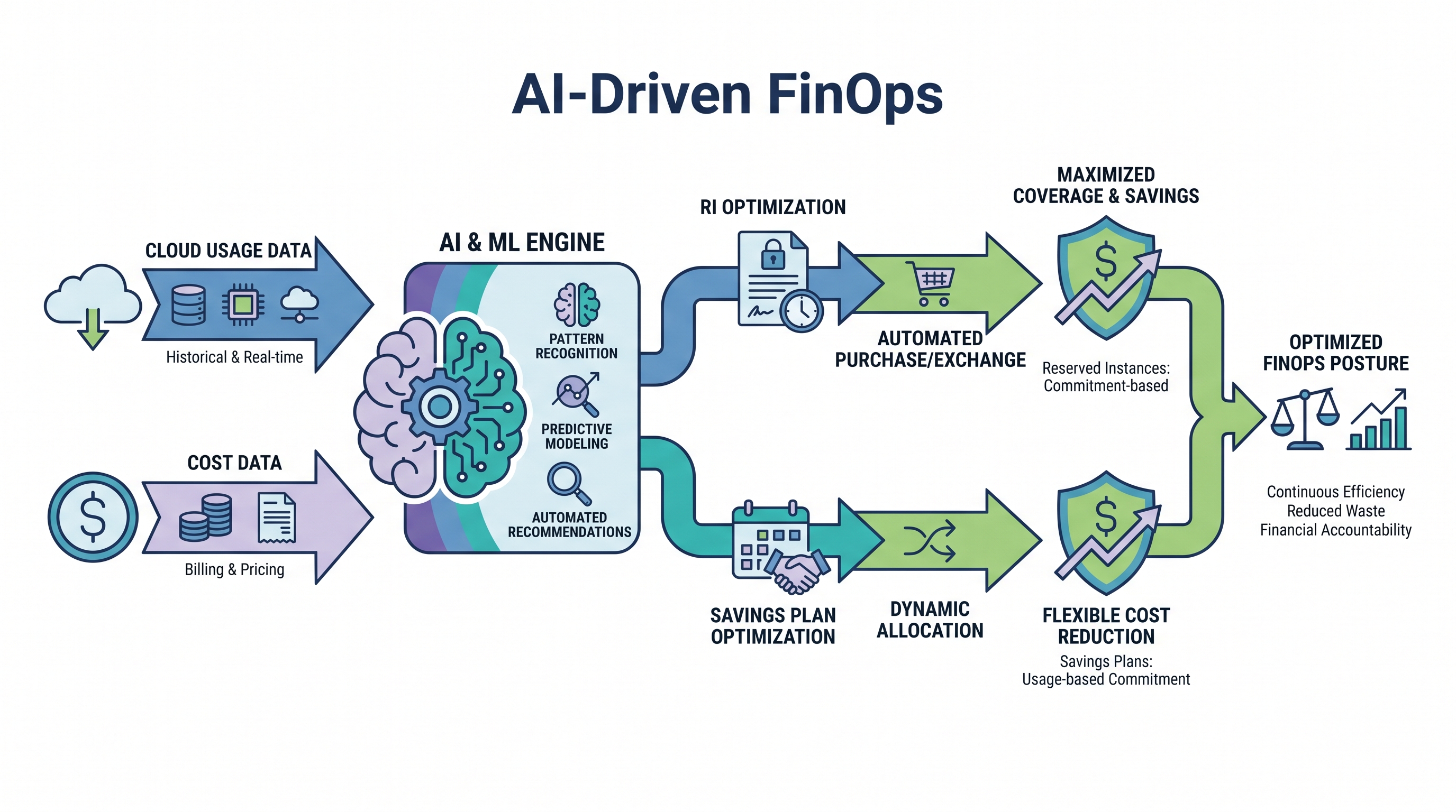
The Multi-Cloud Commitment Dilemma: Beyond Spreadsheets
Modern enterprise cloud architectures are dynamic, highly distributed, and continuously auto-scaling. In environments spanning AWS, Azure, GCP, and Oracle Cloud Infrastructure (OCI), managing compute costs is no longer a task that can be solved with manual spreadsheets or basic heuristic models. Cloud providers offer substantial discounts—often up to 72%—in exchange for long-term capacity commitments via Reserved Instances (RIs) and Savings Plans (SPs). However, the complexity of these commitment mechanisms creates a high-stakes optimization problem.
Commitment instruments vary significantly in their flexibility, scope, and risk profiles:
Standard Reserved Instances: Offer high discounts but are locked to a specific instance family, region, operating system, and tenancy.
Convertible Reserved Instances: Provide slightly lower discounts but allow exchange for different instance types, families, or operating systems within the same region.
Savings Plans (Compute, EC2 Instance, SageMaker): Offer dollar-per-hour commitment flexibility, automatically applying across regions, instance families, and even compute types (e.g., EC2, Fargate, Lambda), but require a rigid 1-year or 3-year term.
The core challenge of FinOps is finding the optimal balance between coverage (the percentage of running resources covered by commitments) and utilization (the percentage of purchased commitments actually used). If your coverage is too low, you waste money on expensive On-Demand rates. If your utilization is too low, you pay for unused commitments, resulting in waste. Manual modeling fails because it cannot scale to thousands of daily micro-decisions, leaving organizations either over-committed (wasting capital) or under-committed (paying premium On-Demand rates). To solve this, organizations must transition to an AI-driven financial operations platform that automates the lifecycle of these commitments.
Architecting an AI-Driven FinOps Engine
To automate RI and SP optimization at scale, we must build a closed-loop engineering architecture. This architecture must continuously ingest raw usage data, process it to extract underlying demand patterns, run mathematical optimization models, and safely execute purchasing decisions through Infrastructure as Code (IaC) or cloud APIs. Below is the reference architecture for an enterprise-grade AI-driven FinOps engine:
+---------------------------------------------------------------------------------+
|                                DATA INGESTION LAYER                             |
|  +------------------+   +-------------------+   +----------------------------+  |
|  | AWS CUR / Parquet|   | Azure Consumption |   | CloudWatch / Prometheus    |  |
|  | (S3 / Athena)    |   | (Blob Storage)    |   | (CPU/Mem Utilization APIs) |  |
|  +--------+---------+   +---------+---------+   +-------------+--------------+  |
+-----------|-----------------------|---------------------------|-----------------+
            |                       |                           |
            v                       v                           v
+---------------------------------------------------------------------------------+
|                          DATA PIPELINE & FEATURE ENGINEERING                    |
|  - Amortization and Normalization                                               |
|  - Trend, Seasonality, and Cyclic Decomposition                                 |
|  - Outlier Detection & Anomaly Suppression (e.g., transient load tests)         |
+-----------------------------------+---------------------------------------------+
                                    |
                                    v
+---------------------------------------------------------------------------------+
|                           MACHINE LEARNING & FORECASTING                        |
|  - DeepAR / LSTM (Time-series prediction of baseline compute demand)             |
|  - Quantile Regression (Risk-aware forecasting: p10, p50, p90)                  |
+-----------------------------------+---------------------------------------------+
                                    |
                                    v
+---------------------------------------------------------------------------------+
|                         MATHEMATICAL OPTIMIZATION ENGINE                        |
|  - Mixed-Integer Linear Programming (MILP)                                      |
|  - Constraints: Expiration dates, budget caps, risk tolerance, regional lock-in |
|  - Portfolio Selector (Optimal mix of Standard RI, Convertible RI, Compute SP)  |
+-----------------------------------+---------------------------------------------+
                                    |
                                    v
+---------------------------------------------------------------------------------+
|                         AUTOMATED EXECUTION & SAFEGUARD LAYER                   |
|  - API Gateway / Cloud SDKs (AWS, Azure, GCP)                                   |
|  - Commitment Intelligence Engine (Purchase validation, change control)          |
|  - Automated Tagging & Guardrails for Rollbacks                                 |
+---------------------------------------------------------------------------------+
The system operates in four continuous stages:
Data Ingestion: Ingests granular cost and usage reports (such as the AWS Cost and Usage Report (CUR) or Azure Consumption Sheets) stored in data lakes (e.g., S3, ADLS) via query engines like Amazon Athena or Snowflake.
Feature Engineering: Cleanses data by stripping out billing anomalies, one-off spikes (such as stress tests or misconfigured deployments), and normalizes different instance sizes to a standard unit (e.g., normalized factor based on vCPU/RAM).
Predictive Modeling: Uses deep learning and time-series models to project future compute demand across different regions, instance families, and operating systems.
Optimization: Solves a multi-variable optimization problem to purchase the exact combination of commitments that yields the highest return on investment (ROI) within specified risk parameters.
Deep Dive: Time-Series Forecasting of Compute Demand
The foundation of any commitment strategy is an accurate forecast of the baseline compute demand. If we model future demand purely on historical averages, we risk over-committing during seasonal traffic drops or under-committing during growth phases. We must predict compute usage at a granular level (e.g., hourly) for the next 30 to 90 days.
Handling Seasonality and Ephemeral Workloads
Cloud workloads typically exhibit multiple overlapping seasonal patterns: daily cycles (peak usage during business hours), weekly cycles (lower usage on weekends), and monthly/quarterly cycles (batch processing or financial close-outs). Ephemeral workloads, such as Auto Scaling groups spinning up for a 2-hour batch job or Kubernetes pods running on spot instances, must be separated from the stable baseline.
To achieve this, we decompose the time-series data $Y(t)$ into trend ($T_t$), seasonal ($S_t$), and residual ($I_t$) components using Seasonal and Trend decomposition using Loess (STL):
Y(t) = T_t + S_t + I_t
The residual component ($I_t$) is analyzed for anomalies. If an anomaly is detected (e.g., a massive spike due to a performance test), it is replaced with an interpolated value based on historical averages to prevent the forecasting model from training on unrepresentative noise.
Quantile Regression for Risk-Aware Forecasting
Standard time-series models (such as ARIMA or standard Prophet) predict the mean expected value. However, in FinOps, predicting the mean is insufficient. If we buy commitments based on the mean forecast, we will be over-committed 50% of the time, resulting in direct financial waste. Instead, we employ Quantile Regression using deep learning architectures like DeepAR or LSTM (Long Short-Term Memory) networks.
By forecasting different quantiles (e.g., P10, P50, P90), we can control our risk appetite:
P10 Forecast (Conservative Baseline): Represents the level of compute usage that we are 90% confident will be exceeded. This is the safest baseline for purchasing 3-year No-Upfront Savings Plans or Standard RIs, as the risk of under-utilization is extremely low.
P50 Forecast (Median Expected Baseline): The point where usage is equally likely to be above or below. This is suitable for flexible, convertible commitments or 1-year plans.
P90 Forecast (High-Water Mark): Represents peak capacity. We should almost never cover the P90 baseline with rigid commitments; instead, this capacity should be handled by a combination of Spot instances, auto-scaling On-Demand instances, or highly flexible Compute Savings Plans.
Implementing this requires a loss function that penalizes over-estimation and under-estimation differently. The Pinball Loss function for a target quantile $\tau$ is defined as:
L_τ(y, ŷ) = max(τ(y - ŷ), (τ - 1)(y - ŷ))
Where $y$ is the actual value and $\hat{y}$ is the predicted value. By setting $\tau = 0.10$, we penalize over-prediction far more severely than under-prediction, forcing the model to output a highly conservative baseline that is ideal for low-risk, high-discount commitments.
The Optimization Engine: Mixed-Integer Linear Programming (MILP)
Once we have generated a risk-aware forecast of compute demand across different regions, instance families, and operating systems, we must decide which commitments to buy. This is a classic operations research problem that can be formulated using Mixed-Integer Linear Programming (MILP).
Formulating the Objective Function
The goal is to minimize the total cost of compute over a given planning horizon (e.g., 12 months). The total cost consists of the amortized cost of commitments purchased, plus the cost of any residual On-Demand usage that is not covered by commitments.
Let:
$I$ be the set of all compute resource configurations (combinations of region, instance family, OS, etc.).
$T$ be the planning time steps (e.g., hourly intervals over 1 year).
$C$ be the set of available commitment options (e.g., 1-year No Upfront Standard RI, 3-year All Upfront Compute SP, etc.).
$x_{i,c}$ be the continuous decision variable representing the quantity of commitment $c \in C$ to purchase for resource configuration $i \in I$.
$OD_{i,t}$ be the continuous variable representing the On-Demand compute capacity used for resource configuration $i$ at time $t$.
$Rate^{OD}_{i}$ be the hourly On-Demand rate for resource $i$.
$Rate^{Commit}_{i,c}$ be the effective hourly rate of commitment $c$ applied to resource $i$.
$Demand_{i,t}$ be the predicted compute demand (e.g., P10 forecast) for resource $i$ at time $t$.
The objective function is to minimize total cost:
Minimize: ∑t ∈ T ∑i ∈ I ( (ODi,t * RateODi) + ∑c ∈ C (xi,c * RateCommiti,c) )
Subject to the following constraints:
Demand Satisfaction: The sum of covered commitments and remaining On-Demand capacity must equal or exceed the predicted demand at every time step $t$:
∑c ∈ C (xi,c * CoverageFactori,c) + ODi,t ≥ Demandi,t (∀ i ∈ I, ∀ t ∈ T)Budget Constraints: The total capital expenditure (CapEx) for upfront payments must not exceed the organization's monthly capital allocation:
∑i ∈ I ∑c ∈ C (xi,c * UpfrontCostc) ≤ MaxUpfrontBudgetRisk Diversification: To prevent over-reliance on a single cloud region or instance type that may become obsolete, we can enforce limits on specific commitment types:
∑c ∈ StandardRI xi,c ≤ α * Demandi,t(where $\alpha \in [0, 1]$ represents the maximum risk-exposure threshold for inflexible commitments).
Solving this system of equations using solvers like Gurobi, COIN-OR CBC, or SciPy's optimization libraries yields a mathematically optimal portfolio. The engine will automatically determine, for instance, that it is cheaper to cover 40% of the baseline with a 3-year Compute Savings Plan, 30% with 1-year Convertible RIs, and leave the remaining 30% to dynamic auto-scaling or Spot instances.
Implementing Automated Execution and Guardrails
A mathematical model is only as good as its execution. In a true automated reserved savings optimization model, the output of the MILP solver is fed directly into an automated execution pipeline. However, auto-purchasing financial commitments carries significant risk if not governed properly.
Architecting Safe Execution Pipelines
To safely automate purchases, organizations must establish a multi-tiered execution pipeline with strict programmatic guardrails:
+---------------------------------------------------------------------------------+
|                                 MILP SOLVER OUTPUT                              |
|                   Recommend Purchase: AWS Compute SP, $50/hr                    |
+---------------------------------------+-----------------------------------------+
                                        |
                                        v
+---------------------------------------------------------------------------------+
|                            PROGRAMMATIC GUARDRAILS                              |
|  - Max purchase step limits (e.g., do not buy more than $10/hr increase at once)|
|  - Minimum utilization threshold verification (current active portfolio > 95%)  |
|  - Drift detection (Is current actual usage diverging from P10 forecast?)      |
+---------------------------------------+-----------------------------------------+
                                        | Passes Guardrails
                                        v
+---------------------------------------------------------------------------------+
|                             MUTATION & API EXECUTION                            |
|  - Generate IAM role session with least-privilege permissions                   |
|  - Call AWS/Azure/GCP Purchasing APIs (e.g., PurchaseSavingsPlans)              |
|  - Log transaction to Audit DB & trigger notification                           |
+---------------------------------------------------------------------------------+
By implementing these programmatic checks, you ensure that even if the forecasting model encounters an unexpected anomaly, the system will fail-safe rather than executing a multi-million dollar, non-refundable commitment. For organizations requiring a comprehensive approach to managing these complex trade-offs, leveraging CIO FinOps solutions provides the necessary executive visibility and governance structures.
Security and Governance in Automated FinOps
Automating financial transactions within a cloud environment introduces unique security risks. The purchasing engine requires highly sensitive IAM permissions (such as savingsplans:PurchaseSavingsPlans or ec2:PurchaseReservedInstancesOffering). If these credentials or roles are compromised, an attacker could execute unauthorized purchases, causing massive financial disruption.
Principle of Least Privilege and IAM Hardening
The automation worker must run on a dedicated execution plane (e.g., an AWS ECS task or a Kubernetes pod) utilizing IAM Roles for Service Accounts (IRSA) or Azure Managed Identities. Under no circumstances should static access keys be stored in code or configuration repositories.
An example of a highly restricted AWS IAM policy for automated Savings Plan purchases is shown below:
{
    "Version": "2012-10-17",
    "Statement": [
        {
            "Sid": "AllowSavingsPlanPurchasesWithLimits",
            "Effect": "Allow",
            "Action": [
                "savingsplans:PurchaseSavingsPlans",
                "savingsplans:DescribeSavingsPlans",
                "savingsplans:DescribeSavingsPlansRates"
            ],
            "Resource": "*",
            "Condition": {
                "NumericLessThanEquals": {
                    "savingsplans:MaxCommitment": "100.00"
                },
                "StringEquals": {
                    "aws:RequestedRegion": "us-east-1"
                }
            }
        },
        {
            "Sid": "DenyAllOtherFinancialActions",
            "Effect": "Deny",
            "Action": [
                "aws-portal:*",
                "billing:Update*"
            ],
            "Resource": "*"
        }
    ]
}
This policy limits the engine to purchasing Savings Plans with a maximum commitment of $100/hour and restricts execution exclusively to the us-east-1 region. This prevents a compromised engine from executing massive, cross-region commitments.
Integrating FinOps and Security Operations
True operational efficiency is achieved when FinOps and security are not treated as separate silos. When optimizing compute resources, the automated engine should coordinate with vulnerability scanning and patch management systems. For instance, if an instance family is identified as obsolete or highly vulnerable, the optimization engine should avoid locking the organization into a long-term Standard RI for that specific family. Instead, it should transition the workload to modern, secure instance types and adjust the commitment portfolio to match.
The CloudAtler Advantage: Unified Cloud Operations
Building, training, and maintaining custom machine learning pipelines and MILP solvers for multi-cloud FinOps is an incredibly resource-intensive task. It requires dedicated teams of data scientists, cloud architects, and financial analysts. CloudAtler eliminates this complexity by providing a unified, AI-powered platform that seamlessly integrates FinOps, cloud security, and automated operations.
With CloudAtler's Atler AI, organizations gain access to a continuous, closed-loop optimization engine that automatically forecasts, models, and executes RI and Savings Plan purchases across AWS, Azure, GCP, and Oracle Cloud. CloudAtler doesn't just look at historical billing data; it correlates cloud spend with real-time performance metrics, security vulnerabilities, and deployment lifecycles, ensuring that every financial optimization decision is secure, compliant, and architecturally sound.
By unifying your operations, CloudAtler delivers:
Automated Commitment Optimization: Continuous, machine-learning-driven adjustments to your RI and SP portfolios to maximize savings and eliminate waste.
Unified Visibility: A single pane of glass across all major cloud providers, combining cost, security, and performance.
Guardrails and Safe Automation: Programmatic safeguards that prevent runaway spend and ensure all automated actions comply with enterprise risk policies.
All in One Place
Atler Pilot decodes your cloud spend story by bringing monitoring, automation, and intelligent insights together for faster and better cloud operations.