The Paradigm Shift: Why Reactive Cloud Scaling Fails the Enterprise

For years, cloud infrastructure teams have relied on reactive auto-scaling policies to maintain application performance. When CPU utilization crosses a 70% threshold, spin up another virtual machine; when queue depth increases, scale out the container fleet. While this reactive model prevents immediate service outages, it introduces severe operational, financial, and security liabilities for enterprise organizations operating at scale across multiple public clouds.

Reactive scaling is fundamentally short-sighted. It treats infrastructure as an infinite, instantly available utility, ignoring the macroeconomic realities of cloud consumption. In a multi-cloud footprint spanning AWS, Azure, GCP, and Oracle Cloud Infrastructure (OCI), reactive scaling leads to:

• Commitment Inefficiencies: Organizations cannot align their 1-year or 3-year Savings Plans, Reserved Instances (RIs), or committed use discounts (CUDs) with real-time fluctuations. This results in either massive waste from over-committed, unused capacity, or exorbitant on-demand charges when demand spikes beyond commitments.

• Storage Bloat and Tiering Failures: Unlike compute, storage does not naturally "scale down." Without predictive insight, data accumulates in expensive, high-performance hot tiers (such as AWS EBS gp3 or Azure Premium SSD v2) long after its active lifecycle has ended, leading to compounding monthly costs.

• Security and Compliance Vulnerabilities: Rapid, unplanned infrastructure expansion increases the attack surface. Security teams struggle to maintain continuous compliance, patch management, and vulnerability scanning when resources are dynamically provisioned and de-provisioned without pre-planned, structured guardrails.

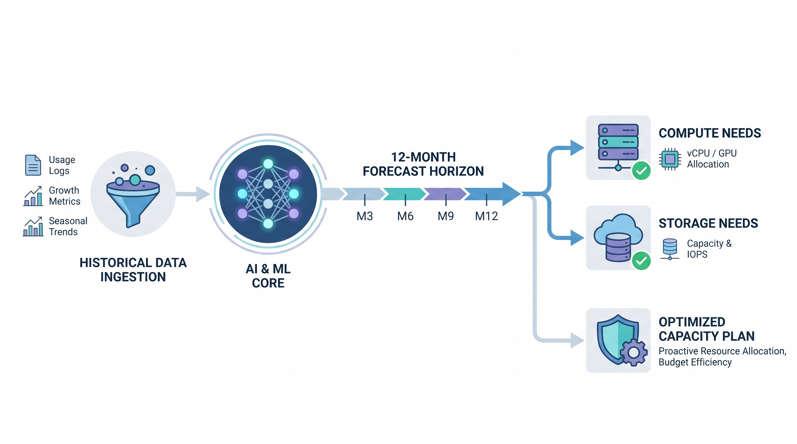
To solve these challenges, forward-thinking enterprises are shifting from reactive scaling to AI-powered capacity planning. By forecasting compute and storage requirements up to 12 months in advance, organizations can transition from a defensive, firefighting posture to a proactive, highly optimized state. This guide provides a deep architectural blueprint for building, training, and operationalizing predictive capacity models across multi-cloud environments.

The Mathematics of 12-Month Predictive Cloud Forecasting

Predicting cloud resource utilization 12 months into the future requires more than simple linear regression. Cloud workloads exhibit complex, non-linear behaviors characterized by daily, weekly, and seasonal patterns, sudden structural breaks (such as product launches or migrations), and long-term macroeconomic trends.

To build an accurate forecasting engine, we must decompose cloud telemetry data into its constituent components. Mathematically, a time-series metric $Y(t)$ (such as CPU core-hours or TB-months) can be modeled as:

Y(t) = T(t) + S(t) + C(t) + e(t)

Where:

• $T(t)$ (Trend): The long-term upward or downward movement in resource consumption, driven by organic business growth, user acquisition, or expanding application footprints.

• $S(t)$ (Seasonality): Periodic fluctuations that repeat over known intervals (e.g., daily batch processing at 02:00 UTC, weekly traffic drops on weekends, or annual holiday shopping spikes).

• $C(t)$ (Cyclical/Event-driven): Non-periodic variations caused by external business events, such as marketing campaigns, system migrations, or sudden architectural changes.

• $e(t)$ (Error/Noise): Unpredictable, random fluctuations that cannot be accounted for by the model.

Evaluating Forecasting Algorithms for Cloud Infrastructure

Different machine learning and statistical models excel at capturing different components of this equation:

For a robust 12-month forecast, a hybrid ensemble approach is often the most effective. For instance, using Prophet to model the baseline trend and macro-seasonality, combined with an XGBoost regressor to adjust for specific business events and metadata-driven variables, yields highly accurate, actionable forecasts.

Architecting the Multi-Cloud Telemetry Data Pipeline

Before applying machine learning models, you must aggregate, clean, and normalize metric data from disparate cloud provider APIs. AWS CloudWatch, Azure Monitor, GCP Stackdriver (Google Cloud Monitoring), and OCI Monitoring all output telemetry in different formats, granularities, and namespaces.

The diagram below outlines the production-grade architecture required to build a unified multi-cloud telemetry pipeline for predictive capacity planning:

+---------------------------------------------------------------------------------+
|                               CLOUD PROVIDERS                                   |
|                                                                                 |
|  [AWS CloudWatch]     [Azure Monitor]     [GCP Stackdriver]     [OCI Metrics]   |
+--------+---------------------+--------------------+--------------------+--------+
         |                     |                    |                    |
         v                     v                    v                    v
+---------------------------------------------------------------------------------+
|                            INGESTION & EXTRACTION LAYER                         |
|                                                                                 |
|   - AWS Metric Streams (Kinesis Firehose)        - Azure Event Hubs             |
|   - GCP Pub/Sub                                  - OCI Streaming Service        |
+---------------------------------------------------------------------------------+
                                       |
                                       v
+---------------------------------------------------------------------------------+
|                            PROCESSING & ETL LAYER                               |
|                                                                                 |
|   - Apache Spark / AWS Glue (Schema Normalization, Timestamp Alignment)         |
|   - Data Cleansing (Handling null values, removing outlier spikes from restarts)|
+---------------------------------------------------------------------------------+
                                       |
                                       v
+---------------------------------------------------------------------------------+
|                            STORAGE & QUERY LAYER                                |
|                                                                                 |
|   - Time-Series Database (e.g., TimescaleDB, Amazon Timestream, or Delta Lake)  |
+---------------------------------------------------------------------------------+
                                       |
                                       v
+---------------------------------------------------------------------------------+
|                            ANALYTICS & FORECASTING                              |
|                                                                                 |
|   - ML Training Pipeline (Prophet / XGBoost Models)                             |
|   - Integration with CloudAtler AI Engine for automated insights                |
+---------------------------------------------------------------------------------+
        

Data Ingestion and Normalization Strategy

To build a clean dataset for your forecasting models, your ETL layer must perform several critical operations:

1. Granularity Alignment: Raw metrics are often collected at 1-minute or 5-minute intervals. For a 12-month forecast, this level of granularity introduces excessive noise and computational overhead. Downsample your metrics to daily averages, maximums, and 95th percentile values. The 95th percentile is particularly crucial for compute capacity planning, as it represents the true peak demand while filtering out anomalous transient spikes.

2. Schema Standardization: Map provider-specific metrics to a unified schema. For example:

   • AWS AWS/EC2/CPUUtilization $\rightarrow$ normalized_cpu_utilization

   • Azure Microsoft.Compute/virtualMachines/Percentage CPU $\rightarrow$ normalized_cpu_utilization

   • GCP compute.googleapis.com/instance/cpu/utilization $\rightarrow$ normalized_cpu_utilization

3. Virtual Machine Metadata Enrichment: Tag telemetry data with instance types, vCPU counts, memory allocations, regions, and business dimensions (e.g., cost center, environment, application owner). This metadata allows the forecasting model to understand the physical resource constraints of the underlying virtual machines.

Forecasting Compute Capacity: Auto-Scaling, Rightsizing, and Lifecycle Analysis

With a normalized telemetry pipeline in place, we can focus on forecasting compute capacity. Compute forecasting is not merely about predicting CPU utilization percentage; it is about predicting the total required resource footprint (vCPUs and Memory GiB-hours) needed to sustain business operations without performance degradation.

The Rightsizing and Lifecycle Conundrum

A common mistake in capacity planning is forecasting the growth of unoptimized infrastructure. If a virtual machine is running at 15% CPU utilization, forecasting its growth over the next 12 months will simply project a larger, equally wasted footprint.

Therefore, any predictive compute capacity framework must integrate continuous rightsizing and a comprehensive compute lifecycle analysis. This analysis evaluates the historical utilization, age, and generation of virtual machine instances. Older generation instances (e.g., AWS m5 or Azure Dsv4) should be flagged for modernization (e.g., upgrading to m7g Graviton or Dsv5) prior to generating long-term forecasts. Modernizing your compute footprint changes the performance-to-cost ratio, which fundamentally alters the resource consumption curve that the AI model must predict.

Python Implementation: Forecasting Compute Growth with Prophet

Below is a production-ready Python snippet illustrating how to train a Prophet model on normalized historical compute telemetry to project vCPU requirements 12 months (365 days) into the future, incorporating business growth factors as an external regressor.

import pandas as pd
from prophet import Prophet

# 1. Load normalized historical telemetry data
# Schema: ds (date), y (vCPU hours utilized), transactions (external business driver)
data = pd.read_csv("multi_cloud_compute_telemetry.csv")
data['ds'] = pd.to_datetime(data['ds'])

# 2. Initialize Prophet model with daily and weekly seasonality
# We include monthly and yearly seasonality to capture long-term enterprise trends
model = Prophet(
    growth='linear',
    yearly_seasonality=True,
    weekly_seasonality=True,
    daily_seasonality=False,
    changepoint_prior_scale=0.05
)

# Add business transaction volume as an external regressor to improve predictive accuracy
model.add_regressor('transactions')

# 3. Fit the model on historical data
model.fit(data)

# 4. Create a future dataframe extending 365 days
future = model.make_future_dataframe(periods=365, freq='D')

# Project external regressor values (transactions) for the next 12 months
# In production, this would come from product/finance team forecasts
future_transactions = []
last_val = data['transactions'].iloc[-1]
for i in range(len(future)):
    if i < len(data):
        future_transactions.append(data['transactions'].iloc[i])
    else:
        # Assuming a conservative 1.5% monthly growth in business transactions
        last_val *= 1.0005 
        future_transactions.append(last_val)

future['transactions'] = future_transactions

# 5. Generate the 12-month forecast
forecast = model.predict(future)

# Extract key metrics: yhat (predicted), yhat_lower/yhat_upper (confidence intervals)
results = forecast[['ds', 'yhat', 'yhat_lower', 'yhat_upper']].tail(365)
print(results.head())

By executing this model across your application portfolios, the output provides three critical data points for your 12-month plan:

• yhat (The Expected Baseline): Use this to purchase 1-year or 3-year Savings Plans or Reserved Instances. This represents the highly probable, steady-state compute requirement.

• yhat_upper (The Peak Capacity Envelope): Use this to establish auto-scaling maximum boundaries and configure infrastructure-as-code (IaC) quotas. This ensures that even during peak demand, your cloud accounts have sufficient limits and resources provisioned.

• yhat_lower (The Minimal Footprint): Use this to identify aggressive rightsizing opportunities. If your actual usage drops to this level, it triggers automated evaluations to downsize or consolidate workloads.

Forecasting Storage Capacity: Hot, Cool, and Archive Tiering Dynamics

Storage capacity planning presents a completely different challenge than compute. While compute utilization is transient, storage is cumulative. Data generated today remains indefinitely unless explicitly deleted or moved down the storage lifecycle hierarchy.

Predictive storage capacity planning must address two distinct vectors: Block Storage (EBS, Managed Disks) and Object Storage (S3, Azure Blob, GCS).

Block Storage: Preventing "Disk Full" Outages and Orphaned Disks

Block storage is directly attached to virtual machines or container nodes. Running out of block storage capacity triggers immediate system instability and application outages. AI-powered capacity models analyze the rate of change in disk write operations (IOPS) and disk space utilization. By calculating the derivative of the storage consumption curve, the predictive engine can project the exact day a disk will reach 90% capacity. This allows SRE teams to expand volumes programmatically during scheduled maintenance windows, eliminating emergency midnight paging events.

Furthermore, block storage forecasting must account for orphaned disks—volumes that remain active and billing long after their associated virtual machine has been terminated. An AI engine trained on multi-resource relationships can flag these orphaned resources, preventing them from skewing the 12-month capacity projection.

Object Storage: Optimizing Tiering with Predictive Lifecycles

Object storage is often the largest cost driver in modern enterprise data lakes. To optimize this, cloud providers offer automated lifecycle policies (e.g., moving objects from S3 Standard to Infrequent Access, and eventually to Glacier Deep Archive). However, static lifecycle policies (e.g., "move to archive after 90 days") are often inefficient because they do not adapt to changing data access patterns.

AI-powered capacity planning analyzes access telemetry—specifically, read-to-write ratios and time-since-last-access metrics. By applying clustering algorithms to these patterns, the system models the decay rate of data utility. The model then predicts the ideal timing for data transition, allowing organizations to optimize their storage tiering strategy 12 months in advance. This prevents the common "retrieval cost shock," where data is archived too early and incurs massive egress fees when recalled for unexpected business analysis.

The Intersection of Capacity Planning, FinOps, and Security

True capacity planning does not operate in an infrastructure silo. It sits at the exact intersection of Financial Operations (FinOps) and Cloud Security.

FinOps Alignment: Commitment Optimization

FinOps is not just about cutting costs; it is about maximizing the business value of every dollar spent in the cloud. A 12-month capacity forecast is the foundational dataset required for advanced rate optimization.

By leveraging predictive data, FinOps teams can confidently execute commitment strategies. For instance, if the 12-month forecast shows a stable baseline of 10,000 vCPUs across AWS and Azure, the organization can purchase 3-year commitments for 8,500 vCPUs (achieving a ~60% discount) and 1-year commitments for another 1,000 vCPUs, leaving only 500 vCPUs to run on-demand or on Spot instances. Without predictive modeling, this level of commitment planning is blind guesswork, often leading to under-utilization or over-spending.

Security and Compliance: Guardrails and Patching Impacts

From a security perspective, unplanned, rapid capacity expansion is a vector for risk. When engineering teams spin up unmonitored shadow IT infrastructure to meet unexpected capacity demands, those resources often lack proper security controls, IAM roles, and patch compliance.

Predictive capacity planning allows security teams to pre-authorize infrastructure blueprints. When the AI models project a capacity expansion in a specific region or business unit, security tools can proactively deploy compliance guardrails, automated vulnerability scanning, and patch intelligence systems to ensure that any new resources are secured from day one. This proactive approach prevents security debt from accumulating as the cloud footprint grows.

Actionable Playbook: Implementing a 12-Month Capacity Plan

To implement an AI-powered capacity planning framework in your organization, follow this step-by-step technical playbook:

Step 1: Establish the Multi-Cloud Data Foundation

Deploy metric collection agents or native cloud-to-cloud connectors to aggregate historical telemetry. You require a minimum of 90 days of historical data to generate a reliable 30-day forecast, and 365 days of historical data to generate an accurate 12-month forecast that accounts for yearly seasonality.

Step 2: Define Your Business Drivers (Regressors)

Work with your product, finance, and business operations teams to identify key business metrics that correlate with infrastructure consumption. Examples include monthly active users (MAU), daily transaction volumes, api call volume, or data ingestion rates. Feed these metrics into your forecasting models as external regressors to align infrastructure growth with actual business growth.

Step 3: Run Continuous Rightsizing and Compute Lifecycle Analysis

Before running your forecast, eliminate existing waste. Use automated tools to perform a comprehensive compute lifecycle analysis, identifying underutilized VMs, obsolete instance families, and orphaned storage volumes. Modernize and rightsize these resources to establish a clean, optimized baseline footprint.

Step 4: Generate the Multi-Horizon Forecast

Deploy your time-series forecasting models (such as the Prophet/XGBoost ensemble detailed above) to generate three distinct forecast horizons:

• Short-Term (1-30 Days): For automated operational scaling, scheduling container workloads, and detecting immediate anomalies.

• Medium-Term (30-90 Days): For tactical rightsizing, storage tiering transitions, and short-term budget alerts.

• Long-Term (90-365 Days): For strategic budget forecasting, multi-cloud commitment planning, and long-range capacity acquisition.

Step 5: Incorporate Uncertainty Planning

No model is 100% accurate. Your capacity planning framework must incorporate uncertainty planning. This means analyzing the variance between your historical forecasts and actual consumption, and using those error metrics to establish dynamic "buffer zones." These buffer zones prevent over-provisioning while ensuring you maintain a safe margin of spare capacity to handle unexpected, catastrophic demand spikes.

Supercharging Capacity Planning with CloudAtler

Building, maintaining, and tuning custom machine learning models and data pipelines across multiple cloud providers is an incredibly complex, resource-intensive endeavor. It requires dedicated data scientists, data engineers, and cloud architects to keep the system running.

CloudAtler simplifies this entire process by unifying FinOps, cloud security, and automated operations into a single, AI-powered platform. Rather than stitching together disparate open-source tools and cloud-native APIs, CloudAtler provides a comprehensive, turnkey solution for enterprise capacity planning.

The Power of the Atler AI Engine

At the core of our platform is the Atler AI engine. This advanced artificial intelligence system automatically ingests telemetry data from AWS, Azure, GCP, and Oracle Cloud, normalizes the metrics, and applies proprietary ensemble forecasting models to project your compute and storage needs 12 months in advance.

Unlike generic forecasting algorithms, the Atler AI engine is specifically trained on cloud infrastructure patterns, allowing it to detect subtle anomalies, identify complex seasonality, and adjust forecasts based on real-world cloud behaviors. It acts as your continuous, automated cloud architect, providing actionable insights without requiring manual feature engineering or model tuning.

Visualizing Your Future with the Financial Command Center

CloudAtler translates complex data science into clear, business-driven insights through our financial command center. This centralized dashboard provides engineering, finance, and security teams with a single source of truth for current and future cloud operations.

Within the Financial Command Center, you can:

• Simulate Scaling Scenarios: Visualize how a 20% increase in user transactions or a planned database migration will impact your multi-cloud spend and resource requirements over the next 12 months.

• Optimize Commitments: Receive automated, precise recommendations for purchasing Savings Plans and RIs based on your 12-month predictive baseline, maximizing your rate optimization with minimal risk.

• Track Security Alignment: Monitor how your predicted capacity expansion aligns with your security posture, ensuring that compliance guardrails and patch management schedules are proactively prepared for incoming infrastructure.

Conclusion: Unify Your Cloud Operations Today

Predictive capacity planning is no longer a luxury reserved for hyperscale tech companies; it is a fundamental requirement for any enterprise operating in the modern multi-cloud landscape. By leveraging AI-powered forecasting models, organizations can eliminate waste, secure their environments, and align their infrastructure spend directly with business growth.

Stop reacting to yesterday's cloud bill or fighting today's emergency capacity outage. It is time to take control of your cloud's future. Join the ranks of high-performing, cost-efficient, and secure enterprises by unifying your cloud operations, security, and FinOps into a single, cohesive strategy.

Ready to see the future of your cloud? Explore the CloudAtler platform today and schedule a personalized demo to discover how AI-powered capacity planning can transform your enterprise operations.