The Reactive Scaling Fallacy: Why Thresholds Fail the Modern Enterprise

For over a decade, cloud architects have relied on reactive autoscaling. The mechanism is simple and universally supported across Amazon Web Services (AWS), Microsoft Azure, Google Cloud Platform (GCP), and Oracle Cloud Infrastructure (OCI): define a metric threshold (e.g., average CPU utilization exceeds 70% for three consecutive evaluation periods of 60 seconds) and trigger a scale-out action. While conceptually elegant, this approach suffers from a fundamental systemic flaw: temporal latency.

When a reactive autoscaling policy is triggered, several sequential phases must occur before the new compute resources can actively process production traffic:

• Detection Latency (1–5 minutes): Metrics must be aggregated and evaluated over a specified time window to avoid false positives from transient spikes.

• Provisioning Latency (1–10 minutes): The cloud provider must allocate physical hardware, initialize the virtual machine (VM) hypervisor or container runtime, and attach network interfaces.

• Bootstrap Latency (30 seconds–5 minutes): The operating system must boot, system daemons must initialize, and configuration management tools (such as Ansible or cloud-init) must run.

• Application Warm-up (10 seconds–3 minutes): Virtual machines running runtime environments like the Java Virtual Machine (JVM) or heavy Python frameworks require warm-up cycles to compile bytecode, initialize connection pools, and populate local caches.

Cumulatively, this reactive scaling lag can range from 3 to nearly 20 minutes. During this window, the existing infrastructure is severely overloaded, leading to dropped TCP connections, highly elevated response latencies, cascade failures, and broken SLAs. Conversely, once the spike subsides, reactive downscaling is often delayed by aggressive cooldown periods to prevent "flapping" (rapidly scaling up and down), resulting in unnecessary compute spend.

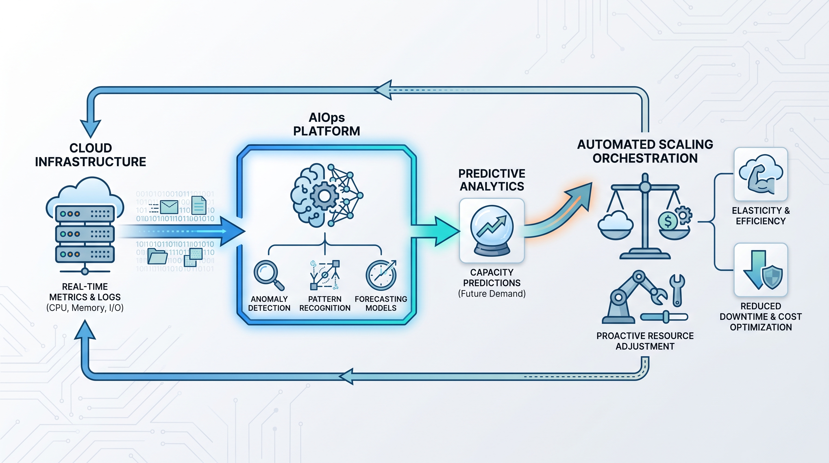
To solve this, modern enterprises are turning to AIOps and machine learning. By utilizing historical telemetry data, organizations can forecast workload demand and trigger scaling actions before the traffic arrives. Implementing these advanced architectures requires a robust predictive monitoring and operations strategy that unifies data collection, model inference, and infrastructure orchestration.

The Architectural Framework of Predictive Autoscaling

Transitioning from reactive to predictive scaling requires shifting from simple event-driven triggers to a continuous feedback loop driven by machine learning. Below is a high-level architectural diagram of a multi-cloud predictive scaling pipeline:

+---------------------------------------------------------------------------------+
|                               INGESTION LAYER                                   |
|  [AWS CloudWatch]     [Azure Monitor]     [Prometheus]     [GCP Cloud Logging]  |
+---------------------------------------+-----------------------------------------+
                                        |
                                        v
+---------------------------------------------------------------------------------+
|                            DATA PIPELINE & STORAGE                              |
|          [Apache Kafka / AWS Kinesis]  -->  [TimescaleDB / InfluxDB]            |
+---------------------------------------+-----------------------------------------+
                                        |
                                        v
+---------------------------------------------------------------------------------+
|                             MACHINE LEARNING ENGINE                             |
|      [Feature Engineering] -> [Model Inference (Prophet/LSTM)] -> [MLflow]      |
+---------------------------------------+-----------------------------------------+
                                        |
                                        v
+---------------------------------------------------------------------------------+
|                           ORCHESTRATION & EXECUTION                             |
|     [CloudAtler Engine] -> [Kubernetes KEDA / Cloud Autoscaling APIs]           |
+---------------------------------------------------------------------------------+
        

1. The Ingestion Layer

The foundation of any ML model is high-fidelity data. In a multi-cloud environment, telemetry must be gathered from disparate sources. This includes system-level metrics (CPU, memory, disk I/O, network throughput), application-level metrics (HTTP request rate, database connection pool exhaustion, queue depth), and external business context metrics (active user sessions, marketing campaign schedules, seasonal indicators). Using unified collectors ensures that data formats are normalized before ingestion.

2. Feature Engineering and Preprocessing

Raw time-series data is rarely ready for model training. The ingestion pipeline must handle missing data points via interpolation, remove anomalies that could skew the model, and construct features that help the model identify patterns. Key features include:

• Lag Features: Metrics from $t-1$, $t-5$, $t-60$ minutes, and $t-1440$ minutes (exactly 24 hours ago) to capture immediate trends and daily patterns.

• Calendar Features: Day of the week, hour of the day, month, and binary indicators for holidays or scheduled business events.

• Rolling Statistics: Rolling means, standard deviations, and exponential moving averages over various window sizes (e.g., 15-minute, 1-hour, and 6-hour windows).

3. The ML Inference Engine

The inference engine runs asynchronously from the core application path. Every 5 to 15 minutes, it pulls the latest metrics, runs them through the trained ML model, and outputs a demand forecast for the next 1 to 4 hours. This forecast is translated into target capacity requirements (e.g., "we will need 45 replicas of the payment service at 14:00 UTC").

4. Orchestration and Execution

The predicted capacity requirements are dispatched to the cloud infrastructure control plane. Rather than relying on standard autoscaling groups, the orchestration layer interacts directly with cloud APIs (such as AWS Auto Scaling, Azure VMSS, or Google Instance Groups) or Kubernetes controllers like KEDA (Kubernetes Event-driven Autoscaling) to provision resources ahead of schedule.

Mathematical and Algorithmic Deep Dive: Selecting the Right ML Model

Choosing the correct mathematical framework is critical to balancing prediction accuracy, computational overhead, and training complexity. Let's analyze three primary machine learning approaches for time-series forecasting in cloud environments.

1. Statistical Models: SARIMAX

Seasonal Autoregressive Integrated Moving Average with Exogenous Regressors (SARIMAX) is a classic statistical model highly effective for univariate time series with clear seasonality and trends. The model is represented as $SARIMAX(p,d,q) \times (P,D,Q)_s$, where:

• $p, d, q$ represent the non-seasonal autoregressive, differencing, and moving average terms.

• $P, D, Q$ represent the seasonal components.

• $s$ represents the seasonal period (e.g., $s=24$ for hourly data with daily seasonality).

Pros: Highly interpretable; requires relatively small datasets to train; performs exceptionally well on stable, highly predictable workloads.

Cons: Struggles with complex, non-linear relationships; computationally expensive to retrain frequently on massive datasets; cannot easily scale to handle thousands of independent microservices simultaneously.

2. Additive Models: Facebook Prophet

Prophet is an open-source forecasting tool designed for analyzing time-series data that displays patterns on different time scales (daily, weekly, yearly). It models time series using an additive framework:

$y(t) = g(t) + s(t) + h(t) + \epsilon_t$

Where:

• $g(t)$ is the trend function modeling non-periodic changes.

• $s(t)$ represents periodic changes (seasonality).

• $h(t)$ represents the effects of holidays or specific events.

• $\epsilon_t$ is the error term representing idiosyncratic changes not accommodated by the model.

Prophet is highly robust to missing data and shifts in the trend, making it an excellent choice for forecasting macro-level cloud resource demands (e.g., predicting daily peak loads across an entire region to optimize pre-purchased commitments).

3. Deep Learning: Long Short-Term Memory (LSTM) Networks

For highly dynamic, non-linear, and high-frequency workloads, Recurrent Neural Networks (RNNs)—specifically LSTMs—are the gold standard. LSTMs solve the vanishing gradient problem of standard RNNs by introducing a memory cell state ($c_t$) controlled by three gates: the input gate ($i_t$), the forget gate ($f_t$), and the output gate ($o_t$).

The mathematical formulation of an LSTM cell at time step $t$ is:

$f_t = \sigma(W_f \cdot [h_{t-1}, x_t] + b_f)$

$i_t = \sigma(W_i \cdot [h_{t-1}, x_t] + b_i)$

$\tilde{c}_t = \tanh(W_c \cdot [h_{t-1}, x_t] + b_c)$

$c_t = f_t c_{t-1} + i_t \tilde{c}_t$

$o_t = \sigma(W_o \cdot [h_{t-1}, x_t] + b_o)$

$h_t = o_t * \tanh(c_t)$

Where $\sigma$ is the sigmoid function, $W$ represents weight matrices, $b$ represents bias vectors, $x_t$ is the input vector, and $h_t$ is the hidden state (output) of the cell.

By feeding sequences of multi-dimensional metrics (e.g., CPU, active connections, and queue latency) into an LSTM, the network can capture complex, non-linear dependencies across multiple time horizons.

Implementing a Predictive Scaling Engine: A Hands-on Python Example

To illustrate the practical implementation of a predictive scaling workflow, let's write a Python script that utilizes historical CPU metric data, trains a forecasting model using Prophet, and generates scaling commands. In a production environment, this engine would run within our Atler AI engine to orchestrate resources automatically.

import pandas as pd
from prophet import Prophet
import requests
import json
import datetime

# Step 1: Ingest telemetry data from your metrics database
# In this example, we assume we have a time-series dataset of CPU utilization
def load_telemetry_data():
    # In practice, query your TimescaleDB or Prometheus API
    # Metrics dataframe must contain 'ds' (datestamp) and 'y' (metric value) columns
    data = {
        'ds': pd.date_range(start='2026-03-01', periods=2016, freq='5min'),
        'y': [50.0 + (15.0 * (i % 288) / 288) + (10.0 * (i % 12 == 0)) for i in range(2016)] # Mock CPU pattern
    }
    df = pd.DataFrame(data)
    return df

# Step 2: Train the Prophet predictive model
def train_predictive_model(df):
    # Initialize Prophet model with daily and weekly seasonality enabled
    model = Prophet(
        growth='linear',
        changepoint_prior_scale=0.05,
        yearly_seasonality=False,
        weekly_seasonality=True,
        daily_seasonality=True
    )
    model.fit(df)
    return model

# Step 3: Generate a forecast for the next 2 hours (24 intervals of 5 minutes)
def generate_forecast(model):
    future = model.make_future_dataframe(periods=24, freq='5min')
    forecast = model.predict(future)
    # Extract the forecasted values for the future window
    predictions = forecast[['ds', 'yhat', 'yhat_lower', 'yhat_upper']].tail(24)
    return predictions

# Step 4: Translate forecasts into scaling decisions
def evaluate_scaling_action(predictions, current_capacity, target_metric_value=70.0):
    # Find the maximum predicted metric value in the next 1 hour (12 intervals)
    max_predicted_load = predictions['yhat_upper'].head(12).max()
    
    # Calculate required capacity based on the predicted load
    # Target capacity formula: current_capacity * (max_predicted_load / target_metric)
    calculated_target = int(round(current_capacity * (max_predicted_load / target_metric_value)))
    
    # Enforce minimum and maximum scaling boundaries
    min_instances = 2
    max_instances = 20
    target_capacity = max(min(calculated_target, max_instances), min_instances)
    
    return target_capacity

# Step 5: Execute scaling action via Cloud API
def execute_scale_out(target_capacity):
    # Example payload to an Orchestrator or Cloud API (e.g., AWS ASG)
    print(f"[{datetime.datetime.utcnow().isoformat()}] Sending scale request to target capacity: {target_capacity} instances.")
    # payload = {"DesiredCapacity": target_capacity, "AutoScalingGroupName": "production-web-asg"}
    # requests.post("https://api.cloudatler.com/v1/scale", json=payload)

if __name__ == "__main__":
    print("Initializing Predictive Scaling Loop...")
    df = load_telemetry_data()
    model = train_predictive_model(df)
    predictions = generate_forecast(model)
    
    current_capacity = 5 # Current active instances
    target = evaluate_scaling_action(predictions, current_capacity)
    
    if target != current_capacity:
        execute_scale_out(target)
    else:
        print("Current capacity matches predicted demand. No action required.")
        

This script demonstrates the logic of a predictive loop. By using the upper bound of the prediction interval (yhat_upper), we build a conservative model that accounts for statistical uncertainty, ensuring that we err on the side of over-provisioning slightly rather than risking an SLA breach.

FinOps Alignment: Optimizing Commitments and Eliminating Waste

Autoscaling is not just an operational concern; it is a core pillar of Financial Operations (FinOps). Uncontrolled scaling can lead to "billing shock" when models react to anomalies or when misconfigured systems scale out horizontally without restraint. Aligning predictive scaling with a structured financial operations platform is essential to maintaining profitability.

The Interplay Between Dynamic Scaling and Cloud Commitments

Enterprise cloud billing relies heavily on commitment-based discounts, such as AWS Savings Plans, Azure Reservations, and GCP Committed Use Discounts (CUDs). These discounts offer significant price reductions (up to 72%) in exchange for committing to a consistent amount of compute usage (measured in $/hour) for a 1- or 3-year term.

This creates a complex optimization challenge. If your baseline compute usage is completely dynamic due to aggressive autoscaling, you may fail to fully utilize your prepurchased commitments, leading to wasted spend. Conversely, if your baseline is set too low, you will run a large percentage of your workloads on expensive On-Demand rates.

Predictive scaling engines solve this by analyzing the long-term trend of your application workloads. By predicting the minimum baseline load over a 30- to 90-day window, the system can provide recommendations for commitment purchasing. This concept, known as commitment intelligence, ensures that your baseline is always covered by high-discount commitments, while the highly variable, predictive scaling spikes are handled using a combination of Spot instances and optimized On-Demand instances.

FinOps Metric Matrix for Predictive Scaling

To measure the efficiency of your predictive scaling model, track the following financial and operational metrics:

Security and Governance in Automated Scaling Environments

When you grant an AI-driven system the authority to provision and terminate infrastructure across multiple cloud providers, you introduce unique security vectors and governance challenges. Without strict guardrails, an exploit or a malformed dataset could lead to massive financial liabilities or service disruptions.

1. Adversarial Scaling Attacks (Billing Exhaustion)

In a traditional Denial of Service (DoS) attack, the goal is to take down the system. In an Adversarial Scaling Attack (or "Economic Denial of Sustainability" - EDoS), the attacker sends carefully crafted, low-frequency traffic patterns designed to mimic the historical scaling triggers of your ML model. By tricking the predictive scaling engine into provisioning maximum capacity across multiple regions, the attacker can silently exhaust your cloud budget without ever triggering traditional security alerts.

To mitigate this threat, organizations must implement strict automated guardrails that sit between the predictive scaling model and the cloud execution APIs. These guardrails must enforce hard limits on maximum daily spend, maximum concurrent instances, and regional expansion rates, regardless of what the ML model predicts.

2. Role-Based Access Control and Policy-as-Code

The predictive scaling engine must operate under the principle of least privilege. Rather than granting the engine broad administrative access to your cloud accounts, construct highly granular IAM roles. For example, in AWS, the engine should only be permitted to execute autoscaling:UpdateAutoScalingGroup and ec2:DescribeInstances on specifically tagged resources.

Furthermore, use Policy-as-Code engines (such as Open Policy Agent or AWS Organizations SCPs) to enforce structural compliance. For example, a policy can mandate that any instance provisioned by the predictive scaling engine must use pre-approved, hardened AMIs that have been scanned by your vulnerability management pipeline.

3. Data Poisoning and Model Drift

Machine learning models are highly susceptible to model drift—the degradation of predictive power over time due to changes in the underlying environment. If an application's codebase changes (e.g., a new release introduces a memory leak), the historical CPU patterns used to train the model are no longer valid. If the model continues to scale based on outdated patterns, it may under-provision resources, leading to a system outage.

To prevent this, implement continuous validation of your model's accuracy. If the Mean Absolute Percentage Error (MAPE) of the predictions exceeds a predefined threshold (e.g., 15%) for three consecutive hours, the orchestration system must automatically fall back to standard, conservative reactive scaling rules while alerting SRE teams to retrain the model.

Unifying Multi-Cloud Operations with CloudAtler

Building, maintaining, and securing a custom, machine-learning-driven predictive scaling engine across AWS, Azure, GCP, and OCI is an immense engineering undertaking. It requires dedicated data science, platform engineering, and FinOps teams to construct data pipelines, manage model lifecycles, and write complex cloud integrations.

CloudAtler simplifies this complexity by providing a unified, AI-powered platform that combines predictive scaling, FinOps optimization, and advanced security guardrails out of the box. With CloudAtler, you can:

• Unify Multi-Cloud Telemetry: Ingest metrics from all major cloud providers and Kubernetes clusters into a single, high-performance data engine.

• Automate Predictive Scaling: Leverage our advanced, pre-trained ML models to forecast resource demand and scale your infrastructure proactively, eliminating the reactive scaling lag.

• Enforce FinOps Guardrails: Protect your budget with intelligent cost-limiting policies, automated commitment optimization, and real-time anomaly detection.

• Secure Your Operations: Ensure compliance with hardened security policies, secure IAM delegation, and continuous vulnerability monitoring of automated workloads.

Don't let reactive scaling lag impact your application performance or inflate your cloud bill. Transcend traditional limitations and unlock the power of true predictive cloud operations.